Getting Started with psAve

Introduction

Propensity score (PS) analyses are only as good as the propensity score model, and in practice the analyst rarely knows which model is right. Logistic regression may miss nonlinearities and interactions; flexible machine learning methods (classification trees, random forests, gradient boosting) capture them but can produce extreme scores and unstable weights. Different candidate models often yield propensity scores that all “look reasonable” yet lead to materially different effect estimates — a form of model dependence that undermines the credibility of the analysis. Rather than committing to a single model, psAve constructs a model-averaged propensity score: a convex combination $\bar e(X) = \sum_m \lambda_m \hat e_m(X)$ of candidate propensity scores, with the mixing weights $\lambda$ chosen on a simplex grid to optimize a balance criterion, implementing the method of Kabata, Stuart & Shintani (2024).

The distinguishing feature of the method is what the mixing weights are asked to balance. Covariate balance criteria treat all covariates as equally important, but for bias in the treatment effect what matters is balance on covariates as they relate to the outcome. The prognostic score — the predicted outcome under the untreated condition, $g(0, X)$ , estimated from untreated units only (Hansen 2008) — summarizes exactly that relationship, and prognostic-score balance has been shown to be a useful diagnostic for propensity score methods (Stuart, Lee & Leacy 2013). psAve takes this one step further and uses the weighted standardized mean difference of a (model-averaged) prognostic score as the selection criterion for the propensity score mixing weights. In the simulations of Kabata, Stuart & Shintani (2024), this “Prog (Ave)” strategy gave the lowest and most robust bias and RMSE across 16 scenarios, compared with single-model propensity scores and with model averaging targeted at prediction accuracy or covariate balance. The result of psave() is deliberately modest: a numeric vector of propensity scores, designed to be handed to MatchIt::matchit() as a distance measure or to WeightIt::weightit() as a propensity score, with balance assessment via cobalt.

Installation

psAve can be installed from GitHub:

# install.packages("remotes")
remotes::install_github("kabajiro/psAve")

The core of the package requires only cobalt (an Import). The candidate learners beyond logistic regression (rpart, ranger, xgboost), as well as MatchIt and WeightIt for the downstream analysis, are Suggests and are only needed when you actually request them.

A matching workflow with the `lalonde` data

We illustrate the paper’s headline estimator — the model-averaged propensity score selected by balance on the model-averaged prognostic score, “Prog (Ave)” — on the lalonde dataset that ships with MatchIt. The estimand is the average treatment effect in the treated (ATT), the package default.

library(psAve)
data("lalonde", package = "MatchIt")

Step 1: Estimate the model-averaged propensity score

psave() looks deliberately like matchit() and weightit(): a treatment formula and a data frame. The one addition is the outcome argument, which names the outcome variable used to build the prognostic score. A one-sided formula (~ re78) reuses the covariates on the right-hand side of formula as the prognostic-model predictors; a two-sided formula (re78 ~ age + educ + ...) lets you specify a distinct prognostic model.

Two of the default candidate learners (ranger and xgboost) are stochastic, so set a seed first for reproducibility:

set.seed(1234)
fit <- psave(treat ~ age + educ + race + married + nodegree + re74 + re75,
             data = lalonde, outcome = ~ re78)

By default this fits four candidate propensity score models ("glm", "rpart", "ranger", "xgboost") and four candidate prognostic models with the same learners, then searches all 1,771 points of the mixing-weight simplex (step 0.05, four candidates). The whole call takes on the order of seconds to a minute on the lalonde data (n = 614), with xgboost dominating the runtime; for a quick first pass you can restrict ps.methods (e.g., ps.methods = c("glm", "rpart")).

fit
#> A psave object (model-averaged propensity score)
#>  - estimand:  ATT
#>  - criterion: prog (weighted ASMD of the model-averaged prognostic score)
#>  - sample:    614 units (185 treated, 429 control)
#> 
#> lambda (PS mixing weights):
#>   glm      0.000  |                    |
#>   rpart    0.000  |                    |
#>   ranger   0.250  |=====               |
#>   xgboost  0.750  |===============     |
#> 
#> gamma (prognostic mixing weights):
#>   glm      0.000  |                    |
#>   rpart    0.000  |                    |
#>   ranger   0.000  |                    |
#>   xgboost  1.000  |====================|
#> 
#> Criterion value at selected lambda: 0.00506
#> 
#> Balance preview (worst covariates + prognostic score):
#>           smd.un smd.wt ks.un ks.wt
#> racewhite  1.882  0.147 0.558 0.044
#> raceblack  1.762  0.131 0.640 0.048
#> re75       0.290  0.105 0.288 0.121
#> prog       0.315  0.005 0.176 0.142
#> 
#> Next:
#>   MatchIt::matchit(treat ~ age + educ + race + married + nodegree + re74 + re75, data = lalonde, distance = x$ps)
#>     or: psave_match(x)
#>   WeightIt::weightit(treat ~ age + educ + race + married + nodegree + re74 + re75, data = lalonde, ps = x$ps, estimand = "ATT")
#>     or: psave_weight(x)

The printout shows the estimand and criterion, the selected mixing weights $\lambda$ (for the propensity score candidates) and $\gamma$ (for the prognostic candidates), the achieved criterion value, a short balance preview, and — importantly — the literal next call you would issue to carry the score into MatchIt.

Step 2: Match on the averaged propensity score

fit$ps is a plain numeric vector, named by the rownames of data, and can be passed directly to MatchIt::matchit() as the distance argument:

m <- MatchIt::matchit(treat ~ age + educ + race + married + nodegree + re74 + re75,
                      data = lalonde, distance = fit$ps,
                      method = "nearest", caliper = .2)

Retyping the formula and the data name creates an opportunity for row misalignment if the two calls do not use literally the same data. The convenience wrapper psave_match() removes that hazard by reusing the formula and data stored in the psave object; all other arguments are forwarded verbatim to matchit(), and the result is an ordinary matchit object:

m <- psave_match(fit, method = "nearest", caliper = .2)
m
#> A `matchit` object
#>  - method: 1:1 nearest neighbor matching without replacement
#>  - distance: User-defined [caliper]
#>  - caliper: <distance> (0.069)
#>  - number of obs.: 614 (original), 104 (matched)
#>  - target estimand: ATT
#>  - covariates: age, educ, race, married, nodegree, re74, re75

Step 3: Assess balance, including prognostic-score balance

Because the object returned by psave_match() is a genuine matchit object, the full cobalt toolkit applies. Supplying the model-averaged prognostic score through distance adds a prognostic-balance row to the balance table — the diagnostic recommended by Stuart, Lee & Leacy (2013):

cobalt::bal.tab(m, distance = data.frame(prog = fit$prog))
#> Balance Measures
#>                 Type Diff.Adj
#> prog        Distance   0.3699
#> distance    Distance   0.2411
#> age          Contin.  -0.2715
#> educ         Contin.  -0.1913
#> race_black    Binary  -0.2308
#> race_hispan   Binary   0.0769
#> race_white    Binary   0.1538
#> married       Binary   0.0385
#> nodegree      Binary   0.0385
#> re74         Contin.   0.2043
#> re75         Contin.   0.2986
#> 
#> Sample sizes
#>           Control Treated
#> All           429     185
#> Matched        52      52
#> Unmatched     377     133

You can also call cobalt::bal.tab() directly on the psave object itself, which assesses balance for the implied inverse-probability weights at the fitted estimand and automatically includes both the averaged propensity score and the prognostic score as distance measures:

cobalt::bal.tab(fit)
#> Balance Measures
#>                Type Diff.Adj
#> ps         Distance   1.1799
#> prog       Distance   0.0051
#> age         Contin.  -0.0897
#> educ        Contin.  -0.0120
#> raceblack    Binary   0.0475
#> racehispan   Binary  -0.0039
#> racewhite    Binary  -0.0437
#> married      Binary  -0.0063
#> nodegree     Binary   0.0339
#> re74        Contin.   0.0294
#> re75        Contin.   0.1050
#> 
#> Effective sample sizes
#>            Control Treated
#> Unadjusted  429.       185
#> Adjusted     36.58     185

Step 4: Estimate the treatment effect

Effect estimation after matching is deliberately not part of psAve — the matched object is a standard matchit object, so all established guidance applies unchanged. We recommend following MatchIt’s vignette on estimating effects after matching (vignette("estimating-effects", package = "MatchIt")), which uses the marginaleffects package to compute the ATT with cluster-robust standard errors on the matched sample. For a weighting analysis instead of matching, including the exact IPW estimator used in the paper, see vignette("weighting", package = "psAve").

Interpreting the output

`print()`

print(fit) is a one-screen orientation: the estimand and selection criterion, the mixing weights rendered as labeled text bars (so you can see at a glance which candidate models contribute to the average), the criterion value at the selected $\lambda$ , a preview of the worst-balanced covariates plus the prognostic score, and the literal next call. A candidate receiving weight 0 was judged not to improve prognostic-score balance; that is informative, not a failure.

`summary()`

summary(fit)
#> Summary of a psave fit
#> Call: psave(formula = treat ~ age + educ + race + married + nodegree + re74 + re75, data = lalonde, outcome = ~re78)
#> 
#> Estimand: ATT;  criterion: prog (weighted ASMD of the model-averaged prognostic score)
#> Sample: 185 treated, 429 control
#> 
#> Selected mixing weights:
#>   lambda (PS):
#>     glm   rpart  ranger xgboost 
#>    0.00    0.00    0.25    0.75 
#>   gamma (prognostic):
#>     glm   rpart  ranger xgboost 
#>       0       0       0       1 
#>   untreated-set MSE of prognostic candidates:
#>      glm    rpart   ranger  xgboost  average 
#> 41000000 33400000 13500000  2580000  2580000 
#> 
#> Criterion value at selected lambda: 0.00506
#> 
#> All criteria, per candidate and for the selected average:
#>         logloss   smd    ks  prog
#> glm       0.397 0.029 0.083 0.099
#> rpart     0.318 0.084 0.065 0.171
#> ranger    0.177 0.099 0.074 0.025
#> xgboost   0.216 0.051 0.055 0.011
#> average   0.202 0.069 0.057 0.005
#> 
#> Balance (covariates + prognostic score):
#>            smd.un smd.wt ks.un ks.wt  
#> age         0.309  0.090 0.158 0.126  
#> educ        0.055  0.012 0.111 0.070  
#> raceblack   1.762  0.131 0.640 0.048 *
#> racehispan  0.350  0.016 0.083 0.004  
#> racewhite   1.882  0.147 0.558 0.044 *
#> married     0.826  0.016 0.324 0.006  
#> nodegree    0.245  0.075 0.111 0.034  
#> re74        0.721  0.029 0.447 0.060  
#> re75        0.290  0.105 0.288 0.121 *
#> prog        0.315  0.005 0.176 0.142  
#> ---
#> '*' = weighted SMD > 0.1

summary(fit) adds three pieces:

Mixing-weight tables for $\lambda$ and $\gamma$ . The $\gamma$ weights tell you which learners the untreated-outcome model relied on (selected by unweighted mean squared error among untreated units).
The diagnostics table: for every single candidate propensity score and for the selected average, all four criteria are reported (log loss, mean weighted ASMD of covariates, mean weighted KS of covariates, and weighted ASMD of the prognostic score). This is the “was averaging worth it?” table — you can verify directly that the averaged score achieves better prognostic-score balance than any single candidate, and see what it trades away (typically a little log loss: the averaged score is usually a worse predictor of treatment than the most flexible single learner, by design).
The full balance table: unweighted versus weighted SMD and KS statistics for every covariate and for the prognostic score, with the conventional 0.1 threshold marked.

`plot()`

plot(fit, type = "balance")
#> Warning in cobalt::love.plot(x = cobalt::bal.tab(x = structure(list(ps = c(NSW1 = 0.623081080701079, : Standardized mean differences and raw mean differences are present in the same
#> plot. Use the `stars` argument to distinguish between them and appropriately
#> label the x-axis. See `love.plot()` for details.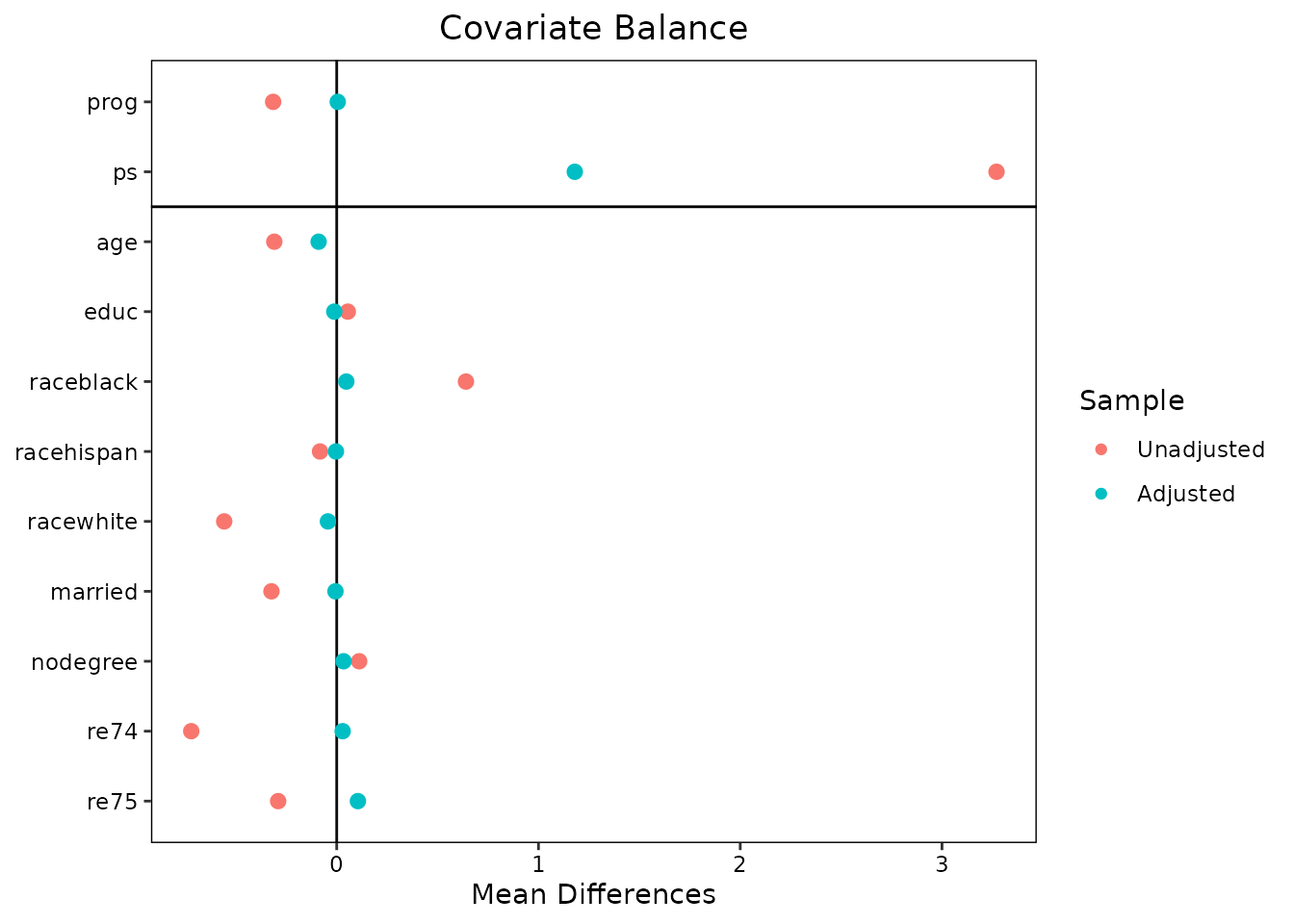

type = "balance" draws a Love plot (via cobalt::love.plot()) of covariate and prognostic-score balance before and after weighting by the implied weights.

plot(fit, type = "distribution")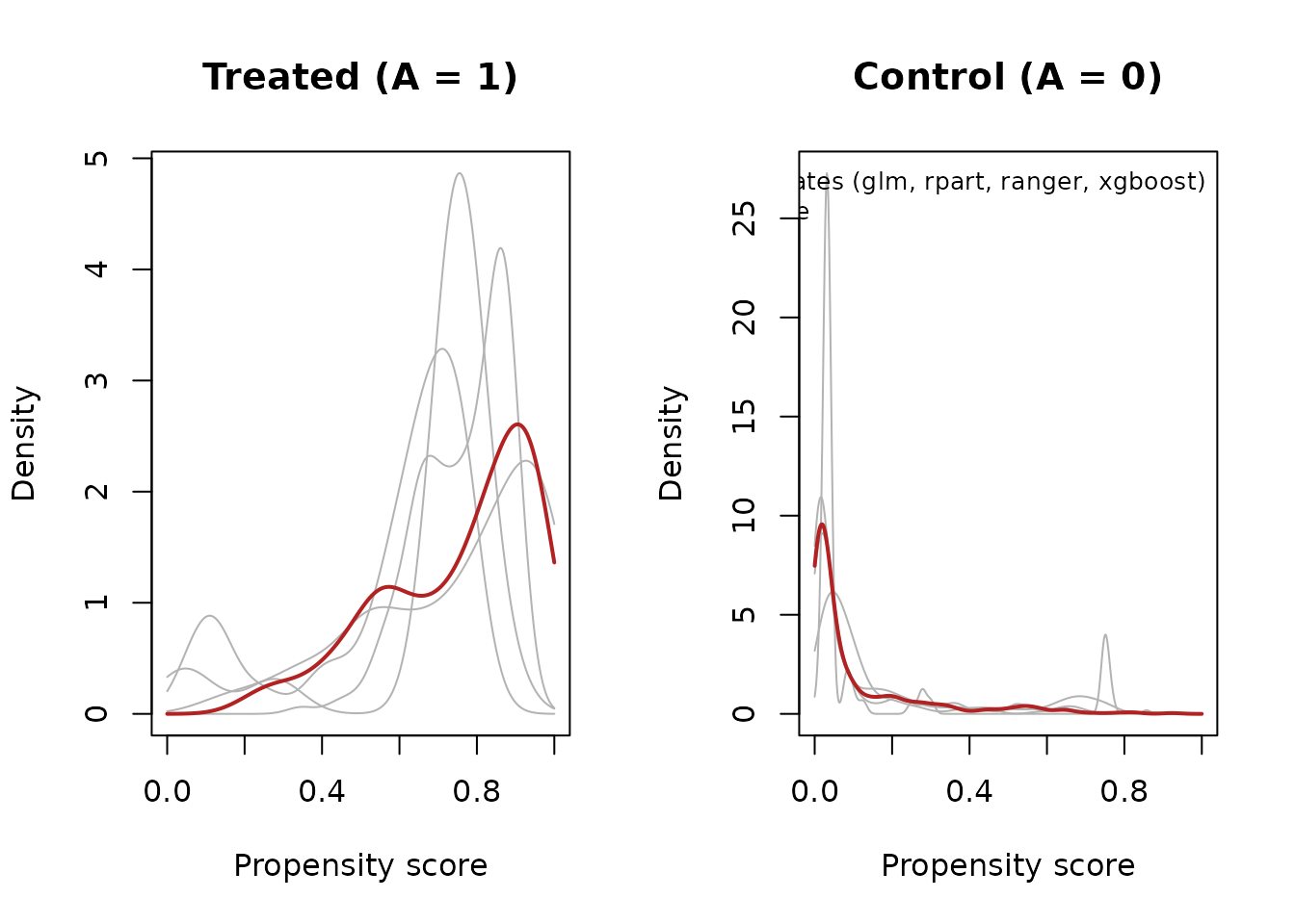

type = "distribution" shows the distribution of the propensity scores by treatment group — each grey curve is one candidate model, and the colored curve is the selected average. This is the plot to inspect for extreme candidate scores: flexible learners fit in-sample can push scores toward 0 or 1 (they are clipped to [0.01, 0.99] by default), and you can see how the averaging tempers them.

plot(fit, type = "criterion")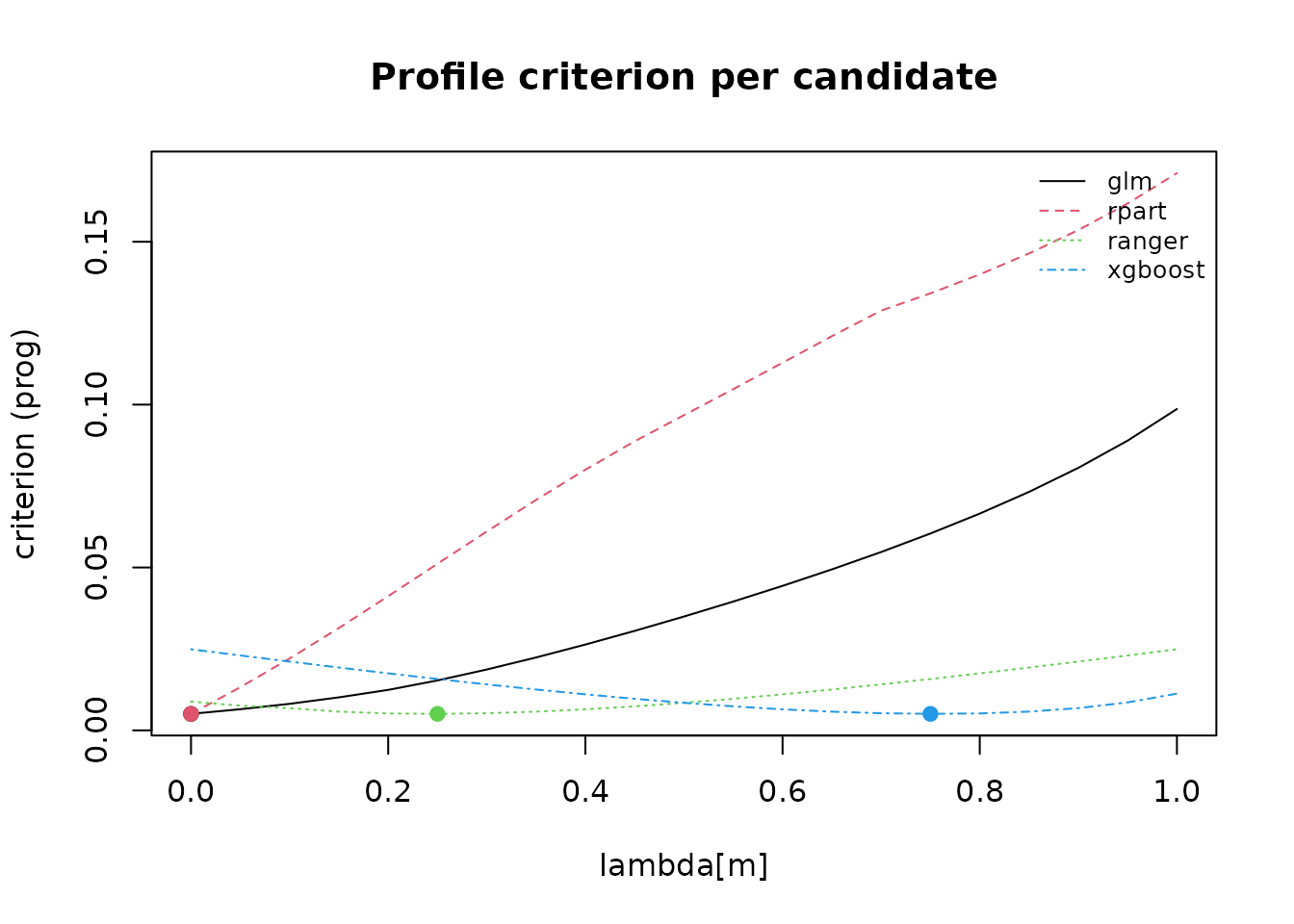

type = "criterion" displays the selection criterion over the $\lambda$ grid (exactly for up to three candidates; as one profile per candidate otherwise), so you can judge how sharply the criterion identifies the selected mixture.

FAQ

Doesn’t using the outcome bias my analysis?

This is the natural first objection, and the design of the method answers it. Two facts matter:

The prognostic model never sees treated outcomes. Following Hansen (2008), the prognostic score $g(0, X)$ is estimated only on untreated units and then predicted for everyone. The $\gamma$ mixing weights are likewise selected using prediction error among untreated units only. No model in the pipeline uses the treated-arm outcomes.
The selection criterion never contrasts outcomes between arms. The $\lambda$ criterion is a balance statistic — the weighted standardized mean difference of the prognostic score between treatment groups. It measures whether the two groups look comparable on an outcome-relevant summary of the covariates; it does not measure, and cannot be driven toward, any particular treatment effect estimate. At no point is a treated-versus-untreated outcome comparison computed during design.

This preserves the separation between the design stage and the analysis stage (Rubin 2001; Hansen 2008): everything psave() does is a function of the covariates, the treatment indicator, and the untreated units’ outcomes, exactly like the prognostic-score balance diagnostics advocated by Stuart, Lee & Leacy (2013). It is the same reasoning under which MatchIt’s documentation welcomes externally estimated distance measures so long as no post-treatment information about the treated-untreated outcome contrast enters the design. A fuller discussion, with the exact formulas, is in vignette("method-details", package = "psAve").

References

Hansen, B. B. (2008). The prognostic analogue of the propensity score. Biometrika, 95(2), 481–488. doi:10.1093/biomet/asn004

Kabata, D., Stuart, E. A., & Shintani, A. (2024). Prognostic score-based model averaging approach for propensity score estimation. BMC Medical Research Methodology, 24, 228. doi:10.1186/s12874-024-02350-y

Stuart, E. A., Lee, B. K., & Leacy, F. P. (2013). Prognostic score-based balance measures can be a useful diagnostic for propensity score methods in comparative effectiveness research. Journal of Clinical Epidemiology, 66(8 Suppl), S84–S90. doi:10.1016/j.jclinepi.2013.01.013

Daijiro Kabata