Getting Started with oalasso

Introduction: which covariates belong in a propensity score model?

A propensity score (PS) model does not need — and should not get — every covariate that predicts treatment. What matters for the treatment-effect estimate is a different set: the confounders (covariates related to both treatment and outcome) and, for efficiency, the pure outcome predictors. Two kinds of covariates should be kept out of the PS model:

Instruments — covariates that predict treatment but are unrelated to the outcome except through treatment. Including them increases the variance of the effect estimate without reducing bias (Brookhart et al. 2006), and, when some confounding remains unmeasured, amplifies the bias that the unmeasured confounding contributes (“Z-bias”; Myers et al. 2011). Strong instruments also push propensity scores toward 0 and 1, creating near-positivity violations and unstable weights.
Noise variables — covariates related to neither treatment nor outcome, which only add variance.

The outcome-adaptive lasso (OAL) of Shortreed & Ertefaie (2017) automates this selection. It fits a logistic PS model with an adaptively weighted lasso penalty, where each covariate’s penalty weight is $|\hat\beta_j|^{-\gamma}$ and $\hat\beta_j$ is that covariate’s coefficient in a linear regression of the outcome on treatment and all covariates. Covariates with no outcome association get an exploding penalty and are forced out of the PS model; confounders and outcome predictors survive. The penalty strength $\lambda_n$ is then tuned by the weighted absolute mean difference (wAMD), a balance criterion that weights each covariate’s post-weighting imbalance by its outcome-coefficient magnitude — so the tuning, like the penalty, is outcome-oriented.

oalasso implements OAL and its elastic-net generalization GOAL (Baldé, Yang & Lefebvre 2023; method = "goal"), on top of glmnet with an exact penalty-scale correction so that the published objectives and tuning grids are reproduced (see vignette("method-details", package = "oalasso")). Like its companion package psAve, the deliverable is deliberately modest: fit$ps is a plain numeric vector of propensity scores, ready for MatchIt::matchit() as a distance measure, WeightIt::weightit() as a propensity score, or psAve::psave() as an appended candidate.

Installation

# install.packages("remotes")
remotes::install_github("kabajiro/oalasso")

The solver (glmnet) and the balance machinery (cobalt) are Imports; MatchIt, WeightIt, and psAve are Suggests, needed only for the corresponding downstream steps.

A first look: instruments are excluded, confounders are kept

A small simulated example in the spirit of Shortreed & Ertefaie’s first scenario makes the selection behavior visible. x1 and x2 are confounders, x3 and x4 predict only the outcome, x5 and x6 predict only treatment (instruments):

library(oalasso)

set.seed(20260702)
n <- 500
X <- matrix(rnorm(n * 6), n, 6, dimnames = list(NULL, paste0("x", 1:6)))
A <- rbinom(n, 1, plogis(X %*% c(1, 1, 0, 0, 1, 1)))
Y <- as.numeric(2 * A + X %*% c(0.6, 0.6, 0.6, 0.6, 0, 0) + rnorm(n))
sim <- data.frame(A, Y, X)

fit.sim <- oal(A ~ x1 + x2 + x3 + x4 + x5 + x6, data = sim, outcome = ~ Y)
fit.sim
#> OAL (Shortreed & Ertefaie 2017, doi:10.1111/biom.12679)
#> An oal object (outcome-adaptive lasso propensity score)
#>  - estimand: ATE;  refit: FALSE (penalized fit)
#>  - sample:   500 units (248 treated, 252 control); 6 covariate column(s)
#>  - selected: delta = -10 (lambda_n = 1.02e-27), gamma = 26
#>  - wAMD at the selection: 0.122
#> 
#> Retained (outcome-related):
#>   x1  (|b| = 0.572)
#>   x2  (|b| = 0.647)
#>   x3  (|b| = 0.600)
#>   x4  (|b| = 0.618)
#> Excluded (outcome-unrelated):
#>   x5  (|b| = 0.00339)
#>   x6  (|b| = 0.06668)
#> 
#> Excluded covariates showed no outcome association; excluding instruments and noise variables from a propensity score model improves precision and avoids bias amplification (Brookhart et al. 2006; Myers et al. 2011).
#> 
#> Next:
#>   MatchIt::matchit(A ~ x1 + x2 + x3 + x4 + x5 + x6, data = sim, distance = x$ps)
#>     or: oal_match(x)
#>   WeightIt::weightit(A ~ x1 + x2 + x3 + x4 + x5 + x6, data = sim, ps = x$ps, estimand = "ATE")
#>     or: oal_weight(x)
#>   ($ps is numeric, named by rownames(sim), strictly inside (0, 1);
#>    it also satisfies psAve::psave(ps.append = cbind(oal = x$ps)).)

The seed is set for the data simulation only: oal() itself is fully deterministic (there is no seed argument because nothing stochastic happens inside).

Reading the printout

The printed output, top to bottom:

Provenance line. The first line always states exactly which published method the fit implements, with its DOI — here "OAL (Shortreed & Ertefaie 2017, doi:10.1111/biom.12679)". Options that leave the validated territory (a binomial outcome model, refit = TRUE, user-supplied outcome.coef) change or extend this label, so the printout is honest about what you can cite; a GOAL fit states whether the lambda2 grid is the author’s published grid (Baldé 2025 supplement) or user-specified.
The selected tuning point. delta is the selected exponent from the lambda grid ( $\lambda_n = n^\delta$ ), gamma the paired penalty exponent, and (for GOAL) lambda2 the selected ridge parameter, together with the achieved wAMD value.
Retained vs excluded covariates. Covariates the penalized PS model kept (“Retained (outcome-related)”) and dropped (“Excluded (outcome-unrelated)”), each with its outcome-coefficient magnitude $|\hat\beta_j|$ — the quantity that drove both the penalty and the tuning. In the simulation above, x5 and x6 (the instruments) land in the excluded list, with a one-line reminder of why exclusion is desirable (Brookhart et al. 2006; Myers et al. 2011).
The literal next call. The printout ends by echoing the exact MatchIt::matchit() call (with your formula and data name) that carries fit$ps forward, or the oal_match(fit) shortcut.

If more than 5% of the propensity scores sit at the clipping bounds (clip = c(0.01, 0.99) by default), the printout appends a near-positivity warning and suggests method = "goal", whose ridge term stabilizes the weights (Jones, Ertefaie & Shortreed 2023).

Workflow 1: matching

The realistic workflow uses the lalonde data from MatchIt. The outcome argument is a one-sided formula naming the outcome variable; the outcome (weight) model always uses the same covariates as the PS model, which is intrinsic to the method:

data("lalonde", package = "MatchIt")

fit <- oal(treat ~ age + educ + race + married + nodegree + re74 + re75,
           data = lalonde, outcome = ~ re78)
fit
#> OAL (Shortreed & Ertefaie 2017, doi:10.1111/biom.12679)
#> An oal object (outcome-adaptive lasso propensity score)
#>  - estimand: ATE;  refit: FALSE (penalized fit)
#>  - sample:   614 units (185 treated, 429 control); 8 covariate column(s)
#>  - selected: delta = -10 (lambda_n = 1.31e-28), gamma = 26
#>  - wAMD at the selection: 877
#> 
#> Retained (outcome-related):
#>   age  (|b| =  128)
#>   educ  (|b| = 1062)
#>   racehispan  (|b| =  560)
#>   racewhite  (|b| =  621)
#>   married  (|b| =  201)
#>   nodegree  (|b| =  126)
#>   re74  (|b| = 1920)
#>   re75  (|b| =  763)
#> Excluded (outcome-unrelated):
#>   (none)
#> 
#> Next:
#>   MatchIt::matchit(treat ~ age + educ + race + married + nodegree + re74 + re75, data = lalonde, distance = x$ps)
#>     or: oal_match(x)
#>   WeightIt::weightit(treat ~ age + educ + race + married + nodegree + re74 + re75, data = lalonde, ps = x$ps, estimand = "ATE")
#>     or: oal_weight(x)
#>   ($ps is numeric, named by rownames(lalonde), strictly inside (0, 1);
#>    it also satisfies psAve::psave(ps.append = cbind(oal = x$ps)).)

fit$ps is a numeric vector named by rownames(lalonde), strictly inside (0, 1), and can be passed directly to matchit() as the distance:

m <- MatchIt::matchit(treat ~ age + educ + race + married + nodegree + re74 + re75,
                      data = lalonde, distance = fit$ps, method = "nearest")

Retyping the formula and data name invites row-misalignment mistakes, so — as in psAve — a thin wrapper reuses the formula and data stored in the fit; all other arguments are forwarded verbatim to matchit() and the result is an ordinary matchit object:

m <- oal_match(fit, method = "nearest", caliper = 0.2)
summary(m)$nn
#>               Control Treated
#> All (ESS)         429     185
#> All               429     185
#> Matched (ESS)     113     113
#> Matched           113     113
#> Unmatched         316      72
#> Discarded           0       0

Note that matching estimates an ATT-type contrast, while oal() tunes the wAMD with ATE weights by default (Shortreed & Ertefaie’s convention — this differs from psave(), whose default estimand is ATT). For a matching analysis you may prefer to align the tuning with the estimand:

fit.att <- oal(treat ~ age + educ + race + married + nodegree + re74 + re75,
               data = lalonde, outcome = ~ re78, estimand = "ATT")
m.att <- oal_match(fit.att, method = "nearest")

Workflow 2: weighting

For inverse probability weighting, oal_weight() hands fit$ps to WeightIt::weightit() as the propensity score, at the fit’s estimand by default:

w <- oal_weight(fit)          # = weightit(..., ps = fit$ps, estimand = "ATE")
summary(w)
#>                   Summary of weights
#> 
#> - Weight ranges:
#> 
#>           Min                                  Max
#> treated 1.172 |---------------------------| 40.071
#> control 1.01  |-|                            4.743
#> 
#> - Units with the 5 most extreme weights by group:
#>                                                 
#>            NSW68  NSW116   NSW10  NSW137  NSW124
#>  treated  13.543  15.986  23.295  23.385  40.071
#>          PSID412 PSID388 PSID196 PSID226 PSID118
#>  control   4.029   4.059   4.239   4.522   4.743
#> 
#> - Weight statistics:
#> 
#>         Coef of Var   MAD Entropy # Zeros
#> treated       1.478 0.807   0.534       0
#> control       0.552 0.391   0.118       0
#> 
#> - Effective Sample Sizes:
#> 
#>            Control Treated
#> Unweighted  429.    185.  
#> Weighted    329.02   58.33

Equivalently, weights(fit) returns the IPW weights implied by fit$ps at the fitted estimand directly, without WeightIt:

head(weights(fit))
#>     NSW1     NSW2     NSW3     NSW4     NSW5     NSW6 
#> 1.565629 4.451580 1.474424 1.288178 1.425257 1.430478

How the tuning works: the wAMD criterion

For each candidate penalty $\lambda_n = n^\delta$ on the grid (lambda supplies the exponents $\delta$ ; the default is Shortreed & Ertefaie’s grid), oal() fits the penalized PS model, forms IPW weights $w_i$ from the clipped scores, and computes the weighted absolute mean difference

$\mathrm{wAMD}(\lambda_n) \;=\; \sum_{j=1}^{p} |\hat\beta_j| \, \left| \frac{\sum_i w_i X_{ij} A_i}{\sum_i w_i A_i} - \frac{\sum_i w_i X_{ij} (1 - A_i)}{\sum_i w_i (1 - A_i)} \right|,$

summed over all covariate columns (on the standardized scale), including those the model excluded. The grid point minimizing wAMD is selected. Because each covariate’s imbalance is weighted by its outcome-coefficient magnitude $|\hat\beta_j|$ , residual imbalance on an instrument (with $\hat\beta_j \approx 0$ ) costs almost nothing — the criterion deliberately does not reward balancing covariates that cannot cause confounding. Each $\delta$ is paired with a penalty exponent $\gamma = 2(2 - \delta + 1)$ so that the pair satisfies the method’s theoretical rate conditions; vignette("method-details", package = "oalasso") gives the formulas, the provenance of every default, and the exact glmnet correction that makes the published objective reproducible.

The criterion path is stored and plottable:

plot(fit, type = "wamd")

and oal_wamd() — the exported single source of truth for the criterion — scores any candidate propensity score on the same formula, which is convenient for comparing an OAL score against an external one.

`summary()`, balance, and the other accessors

summary(fit)
#> OAL (Shortreed & Ertefaie 2017, doi:10.1111/biom.12679)
#> Summary of an oal fit
#> Call: oal(formula = treat ~ age + educ + race + married + nodegree + re74 + re75, data = lalonde, outcome = ~re78)
#> 
#> Estimand: ATE;  criterion: wamd (weighted absolute mean difference);  refit: FALSE
#> Sample: 185 treated, 429 control
#> Selected: delta = -10 (lambda_n = 1.31e-28), gamma = 26;  wAMD = 877
#> 
#> Selection table (outcome coefficients on the standardized scale):
#>         term outcome.coef penalty.factor   coef selected     role
#> 1        age      128.234       1.56e-55  0.016     TRUE retained
#> 2       educ     1061.689       2.11e-79  0.161     TRUE retained
#> 3 racehispan      560.127       3.50e-72 -2.082     TRUE retained
#> 4  racewhite      620.617       2.44e-73 -3.065     TRUE retained
#> 5    married      200.536       1.39e-60 -0.832     TRUE retained
#> 6   nodegree      125.523       2.71e-55  0.707     TRUE retained
#> 7       re74     1919.923       4.31e-86  0.000     TRUE retained
#> 8       re75      763.035       1.13e-75  0.000     TRUE retained
#> 
#> Best grid row per lambda2 (by wAMD):
#>   lambda2 delta lambda.n gamma        s wamd n.selected refit.converged
#> 1      NA   -10 1.31e-28    26 1.14e-86  877          8              NA
#>   selected
#> 1     TRUE
#> 
#> Outcome (weight) model: lm(y ~ A + X)
#>           term estimate  se
#> 1  (Intercept)     6330 366
#> 2            A     1550 781
#> 3          age      128 321
#> 4         educ     1060 418
#> 5   racehispan      560 328
#> 6    racewhite      621 385
#> 7      married      201 343
#> 8     nodegree      126 409
#> 9         re74     1920 377
#> 10        re75      763 345
#> 
#> Balance (original-scale covariates):
#>            smd.un smd.wt ks.un ks.wt  
#> age         0.242  0.168 0.158 0.191 *
#> educ        0.045  0.130 0.111 0.077 *
#> racehispan  0.277  0.016 0.083 0.005  
#> racewhite   1.408  0.138 0.558 0.055 *
#> married     0.721  0.210 0.324 0.094 *
#> nodegree    0.235  0.116 0.111 0.055 *
#> re74        0.596  0.274 0.447 0.312 *
#> re75        0.287  0.158 0.288 0.153 *
#> ---
#> '*' = weighted SMD > 0.1

summary() shows the full per-covariate selection table (fit$selected: outcome coefficient, penalty factor, PS coefficient, retained/excluded role), a summary of the tuning path, the outcome-model coefficient table, and a covariate balance table (fit$balance: unweighted and weighted SMD and KS statistics, computed by cobalt with the selected weights — the same layout as psave$balance).

Balance is also available through the cobalt generic, and as a Love-style plot:

cobalt::bal.tab(fit)
#> Balance Measures
#>                Type Diff.Adj
#> ps         Distance   0.1361
#> age         Contin.  -0.1675
#> educ        Contin.   0.1296
#> racehispan   Binary   0.0047
#> racewhite    Binary  -0.0546
#> married      Binary  -0.0944
#> nodegree     Binary  -0.0547
#> re74        Contin.  -0.2740
#> re75        Contin.  -0.1579
#> 
#> Effective sample sizes
#>            Control Treated
#> Unadjusted  429.    185.  
#> Adjusted    329.02   58.33
plot(fit, type = "balance")
#> Warning in cobalt::love.plot(x = cobalt::bal.tab(x = structure(list(ps = c(NSW1 = 0.638720962917443, : Standardized mean differences and raw mean differences are present in the same
#> plot. Use the `stars` argument to distinguish between them and appropriately
#> label the x-axis. See `love.plot()` for details.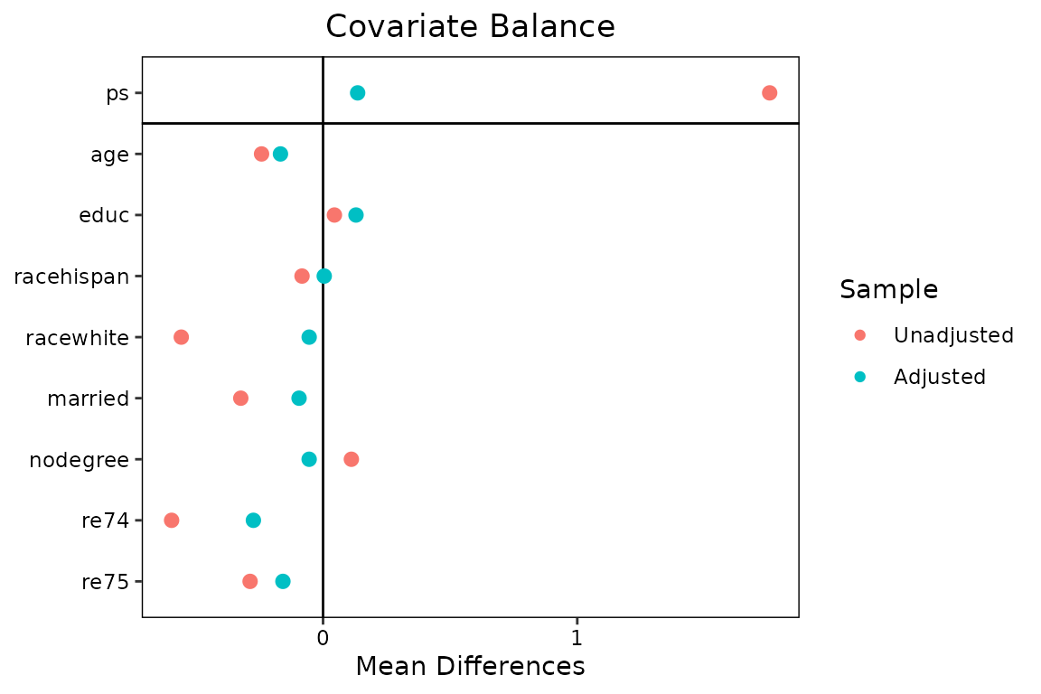

Further accessors: coef(fit) (PS coefficients, original or standardized scale), predict(fit, newdata) (propensity scores for new data, no refitting machinery needed), and fit$path / fit$sets / fit$coef.path for the full grid history (kept unless keep.path = FALSE).

GOAL, in one paragraph

When covariates are strongly correlated or positivity is fragile, plain OAL can select erratically among correlated confounders and produce unstable weights. method = "goal" adds an elastic-net ridge term $\lambda_2 \sum_j \alpha_j^2$ to the objective (Baldé, Yang & Lefebvre 2023), selected jointly with $(\lambda_n, \gamma)$ by the same wAMD criterion; lambda2 = 0 is always on the grid, so GOAL nests plain OAL and can never do worse on the criterion. The default lambda2 grid is the author’s published grid (Baldé 2025 supplement, “taken from Zou and Hastie (2005)”), and the printed provenance line says so. See the method-details vignette.

fit.goal <- oal(treat ~ age + educ + race + married + nodegree + re74 + re75,
                data = lalonde, outcome = ~ re78, method = "goal")

Practical policies worth knowing

Missing data are an error, never a silent drop. Any NA in the treatment, the PS covariates, or the outcome variable stops with a message naming the offending variables. Impute first if that is your analysis plan.
Everything is deterministic. Same data, same arguments, same result — there is no seed argument.
Using the outcome at the design stage is by design. OAL uses outcome coefficients to decide which covariates to select, not to pick the estimate you like; the treatment-effect estimation itself stays downstream in MatchIt/WeightIt/survey/marginaleffects.

Where to go next

vignette("psave-integration", package = "oalasso") — appending the OAL score as a candidate in psAve::psave(), when that composition helps, and its caveats.
vignette("method-details", package = "oalasso") — all formulas, the exact glmnet penalty-scale correction, the provenance of every default, differences from the author’s legacy code, and honest notes on nonlinear extensions.

References

Baldé, I., Yang, Y. A., & Lefebvre, G. (2023). Reader reaction to “Outcome-adaptive lasso: Variable selection for causal inference” by Shortreed and Ertefaie (2017). Biometrics, 79(1), 514–520. doi:10.1111/biom.13683

Brookhart, M. A., Schneeweiss, S., Rothman, K. J., Glynn, R. J., Avorn, J., & Stürmer, T. (2006). Variable selection for propensity score models. American Journal of Epidemiology, 163(12), 1149–1156. doi:10.1093/aje/kwj149

Jones, J., Ertefaie, A., & Shortreed, S. M. (2023). Rejoinder to “Reader reaction to ‘Outcome-adaptive lasso: Variable selection for causal inference’ by Shortreed and Ertefaie (2017)”. Biometrics, 79(1), 521–525. doi:10.1111/biom.13681

Myers, J. A., Rassen, J. A., Gagne, J. J., Huybrechts, K. F., Schneeweiss, S., Rothman, K. J., Joffe, M. M., & Glynn, R. J. (2011). Effects of adjusting for instrumental variables on bias and precision of effect estimates. American Journal of Epidemiology, 174(11), 1213–1222. doi:10.1093/aje/kwr364

Shortreed, S. M., & Ertefaie, A. (2017). Outcome-adaptive lasso: Variable selection for causal inference. Biometrics, 73(4), 1111–1122. doi:10.1111/biom.12679

Daijiro Kabata